How to write basic pipelines

Pipelines explains in more detail what pipelines are, whereas this page will look at some practical examples.

Before we start

This tutorial is aimed at people who have used RiskScape models a lot, and now want to start creating more customized pipelines of their own. We expect that you:

Have been through the How to write RiskScape expressions tutorial already.
Are comfortable writing basic RiskScape expressions.
Are comfortable using RiskScape commands from the terminal prompt.

The aim of this tutorial is to give you enough knowledge to take a pipeline generated by the wizard and start adding extra pipeline steps of your own.

Tip

To learn more about creating bookmarks, writing functions, or defining types, please refer to the Creating a RiskScape project tutorial. Functions and bookmarks are separate concepts that apply regardless of whether you build your model in the wizard or write a pipeline from scratch.

Setup

Click here to download the input data we will use in these examples. Unzip the file into a new directory, e.g. C:\RiskScape_Projects\.

Open a command prompt and cd to the directory where you unzipped the files, e.g.

cd C:\RiskScape_Projects\pipeline-basics

You will use this command prompt to run the RiskScape commands in this tutorial.

The unzipped directory contains an empty file called pipeline.txt. Open this file in a text editor, such as Notepad or gedit. This is where you will paste the pipeline examples.

The project.ini is pretty simple - it loads the pipeline.txt contents as a pipeline model called tutorial.

Open the buildings.csv file and familiarize yourself with the data. This is the building input data we will use in our pipeline.

Note

This tutorial will focus on general pipeline concepts that make up part of a RiskScape model. For simplicity, the buildings do not have any geospatial data associated with them. We will focus on simply transforming the input data, rather than constructing an actual risk model from scratch.

The basics

A RiskScape pipeline is simply a series of data processing steps. Each step in the pipeline has one particular job to do, which is reflected in the step’s name.

The output data from one pipeline step becomes the input data for the next pipeline step. By chaining steps together, we can achieve complex data processing tasks, such as a risk analysis model.

For example, previous tutorials have looked at how you can use aggregation to collate or group your results.

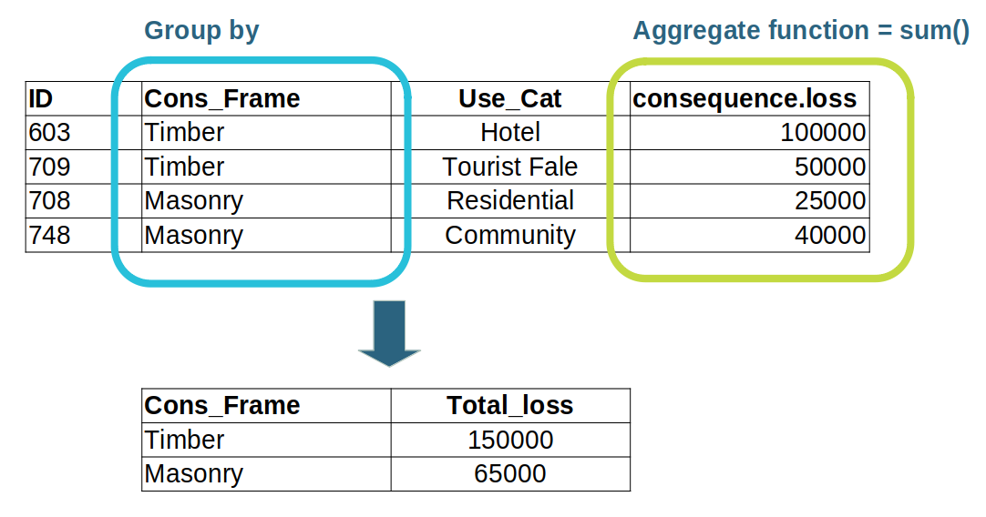
Four rows of building data are aggregated down to two rows, by grouping on the building construction type.

This aggregation operation is actually achieved by a group pipeline step, which we will learn more about soon. The aggregation operation transforms the rows of input data, or tuples. In this case, the output data from the pipeline step looks quite different to the step’s input data.

Input data

Let’s start off with the simplest possible case: loading your data into RiskScape. Every pipeline starts off with an input step that specifies the bookmark data to use.

Add the following to your pipeline.txt file and save it.

input('buildings.csv')

Now try running the pipeline using the following command.

riskscape model run tutorial

The command should produce an output file called input.csv in a time-stamped output/tutorial/ sub-directory.

Note

At the end of the pipeline, the pipeline data is always saved to file. By default, the filename will correspond to the name of the last pipeline step, which is input in this case.

Open the input.csv file that was produced and check its contents.

Tip

Entering more "<filename>" into the command prompt is a quick way to check a file’s contents.

You should see that the output file has the exact same content as the buildings.csv input file. This is because we loaded the data into the pipeline, but we did nothing with it.

Don’t worry, we’ll start doing more complicated things with the input data soon.

Pipeline parameters

You may notice that the input('buildings.csv') syntax looks a lot like a function call. The bit inside the brackets are called the pipeline step parameters. The parameters specify how the step processes the pipeline data it receives.

Each pipeline step comes with some basic documentation that will help you understand how to use it. You can read this help documentation using riskscape pipeline step info STEP_NAME. You can see a list of supported pipeline steps using riskscape pipeline step list.

Try reading about the parameters that the ‘input’ step takes.

riskscape pipeline step info input

Similar to function arguments, the pipeline step parameters have keyword names, e.g.

input(relation: 'buildings.csv')

If a pipeline step has many optional parameters, then you will have to use the parameter keywords.

Note

You will notice that the relation parameter in the input step can be a bookmark or filename/URL. We are using the filename here because we haven’t defined any bookmarks at all. In this case, the file path is relative to the directory that our project.ini file is in.

Adding a filter step

Now we will add in a second pipeline step to actually do something with the input data.

Let’s say we want to exclude any Outbuildings from our data. Replace the contents of your pipeline.txt file with the following.

input('buildings.csv')
  ->
filter(Use_Cat != 'Outbuilding')

The filter step takes a boolean (true or false) conditional expression. When the condition evaluates to true for a row of data, that row will be passed onto the next pipeline step. When the condition evaluates to false, that row of data will be excluded from the pipeline.

The -> is used to chain two pipeline steps together. Think of it as representing the input data flowing between the two steps.

Try running this pipeline using the following command:

riskscape model run tutorial

This should produce a filter.csv output file. Notice that the name of the output file has changed to match the last step in our pipeline.

Open the filter.csv output file and check its contents. The pipeline has now transformed the input data so there are no longer any Outbuildings included.

Transforming data with select

We have seen that the filter step can remove rows of input data. Now let’s try manipulating each row of input data a little. The select pipeline step will be the main way you transform the attributes in your data.

The select step is a lot like the SELECT SQL statement (without the WHERE clause). It tells RiskScape which attributes (columns) to pull out of the rows of input data.

Let’s try a really simple select step. Replace the contents of your pipeline.txt file with the following.

input('buildings.csv')
  ->
filter(Use_Cat != 'Outbuilding')
  ->
select( { ID, Use_Cat, Cons_Frame as construction, REGION } )

Save pipeline.txt and enter the following command to run your latest pipeline.

riskscape model run tutorial

This time it will produce a select.csv output file. Open this file and examine its contents.

The select step actually did several things:

It reordered the Use_Cat and Cons_Frame columns.
It renamed the Cons_Frame attribute to construction.
It removed the storeys and area attributes from the input data, because these were not specified in the select at all.

You may have noticed that this time the pipeline code contains { }s. This is because the select step actually takes a Struct expression as its parameter.

Note

Each row of data, or tuple, in the pipeline is actually an instance of a Struct. The select step is simply building the Struct that the next pipeline step will receive.

Adding new attributes

Now we will try another simple example where we create a new attribute and add it to our pipeline data. Let’s say we want to approximate the total floor-space in the building by taking the area of the building footprint and multiplying it by the number of storeys it has.

Replace the contents of your pipeline.txt file with the following. Note that we have split the Struct declaration in the select step over several lines here, so that it is easier to read.

input('buildings.csv')
  ->
filter(Use_Cat != 'Outbuilding')
  ->
select({
         Use_Cat,
         Cons_Frame as construction,
         REGION,
         storeys * area as floorspace
       })

Now try running the pipeline model again using the following command:

riskscape model run tutorial

Uh-oh, something went wrong this time.

Failed to validate model for execution
  - Failed to validate 'select({Use_Cat, Cons_Frame as construction, REGION, storeys * area as floorspace})' step for execution
    - Failed to validate expression '{Use_Cat, Cons_Frame as construction, REGION, storeys * area as floorspace}' against
      input type {ID=>Text, Cons_Frame=>Text, Use_Cat=>Text, area=>Text, storeys=>Text, REGION=>Text}
      - Operator '*' is not supported for types '[Text, Text]'

Remember that RiskScape uses indentation to show how the errors are related - they drill-down in more and more specific detail about the actual problem. The first error tells us the problem was with the select step. The next line tells us there was something wrong with our Struct expression. Finally the last error tells us the problem was with the multiplication part of the expression - we are trying to multiply two Text strings.

You may recall that everything in RiskScape has a type, and CSV data is always Text type. So here we need to tell RiskScape that these attributes are actually Integer values. Normally you would do this in your bookmark, but because we are not using bookmarks at all, we can call casting functions instead to turn the Text strings into Integer and Floating values.

Update your pipeline.txt file to contain the following:

input('buildings.csv')
  ->
filter(Use_Cat != 'Outbuilding')
  ->
select({
         Use_Cat,
         Cons_Frame as construction,
         REGION,
         int(storeys) * float(area) as floorspace
       })

Save the file and run the pipeline model again using the following command:

riskscape model run tutorial

Check that the command works now, and a new floorspace attribute is included in the new output file.

Tip

Using int() and float() here are function calls. Remember that you can call a function from any RiskScape expression, and calling functions allows you to do much more complicated things in your pipeline. The select step is a great place to call functions, although you can call functions from any pipeline step that accepts expression parameters.

Naming steps

Each step in the pipeline has a name. So far we have been relying on RiskScape to use a default name for us.

You specify the pipeline step name by adding as YOUR_STEP_NAME after the closing ) bracket. Let’s try naming the select step now.

input('buildings.csv')
  ->
filter(Use_Cat != 'Outbuilding')
  ->
select({
         Use_Cat,
         Cons_Frame as construction,
         REGION,
         int(storeys) * float(area) as floorspace
       }) as calc_floorspace

If you run the pipeline again, you will notice that the output filename now matches the name of the last step in our pipeline.

Tip

You don’t have to worry too much about naming your pipeline steps unless you want to ‘fork’ a pipeline chain into two (i.e. to create multiple output files), or combine two separate pipeline chains together (i.e. to combine input data from different files).

Select all attributes

It can get a bit cumbersome in select steps to always specify every single attribute that you want to retain. Luckily, there is an easier way to do this when you are only adding new attributes to the pipeline data.

When used on its own in a Struct expression, the * operator acts as a wildcard that means include all attributes.

Let’s say we also want to convert the floor-space (in square metres) to square feet. Try running the following pipeline.

input('buildings.csv')
  ->
filter(Use_Cat != 'Outbuilding')
  ->
select({
         Use_Cat,
         Cons_Frame as construction,
         REGION,
         int(storeys) * float(area) as floorspace
       }) as calc_floorspace
  ->
select({
         *,
         round(floorspace * 10.76) as square_footage
       })

Check the output file that gets produced. All the attributes produced by the previous calc_floorspace step should still be there, as well as the new square_footage attribute.

Note

We also used the round() function here to round the square_footage value to the nearest whole number.

Aggregation

Aggregation lets you combine many rows of data into a single result, or group of results, such as the total floor space across all buildings. Aggregation works a lot like a GROUP clause in SQL.

Now let’s try aggregating the buildings by their construction type to calculate some statistics about our buildings. To aggregate the rows of data into a combined result, we use the group step.

The select step transforms each row of data one at a time. Whereas the group aggregation works across all rows of data.

The group pipeline step takes two parameters:

by: the attribute(s) that we are grouping by (i.e. the construction type).
select: a Struct expression that specifies what aggregation to include in the output.

Try running the following pipeline and check the output results.

input('buildings.csv')
  ->
filter(Use_Cat != 'Outbuilding')
  ->
select({
         Use_Cat,
         Cons_Frame as construction,
         REGION,
         int(storeys) * float(area) as floorspace
       }) as calc_floorspace
  ->
select({
         *,
         round(floorspace * 10.76) as square_footage
       })
  ->
group(by: construction,
      select: {
                construction as "Building type",
                sum(square_footage) as total_square_footage,
                count(*) as Num_buildings
              })

This should now produce a group.csv output file that looks like the following:

Building type,total_square_footage,Num_buildings
Reinforced Concrete,85340,13
Timber,236298,320
Masonry,4574663,2211
Steel,15949,7
Reinforced_Concrete,128368,10

Instead of having a row of data for each building, we now have one row of data for each building type.

The select parameter looks very similar to the select pipeline step. However, the difference here is that the Struct contains aggregation expressions.

Tip

Aggregation expressions always apply across all rows. You can think of the sum(square_footage) expression in RiskScape as like using the SUM() spreadsheet formula across the whole square_footage column.

Note

You may have also noticed that we used double-quotes around "Building type". When an attribute identifier contains non-alphanumeric characters, such as spaces or - dashes, it needs to be enclosed in double-quotes.

Aggregating by multiple attributes

Often you will want to aggregate your results by multiple attributes, e.g. by construction-type and by region. To do this, all we need to do is specify the by parameter as a Struct expression containing all the attributes we are interested in.

For example, let’s try aggregating by construction type and the region that the building is in. Try running the following pipeline and check the results.

input('buildings.csv')
  ->
filter(Use_Cat != 'Outbuilding')
  ->
select({
         Use_Cat,
         Cons_Frame as construction,
         REGION,
         int(storeys) * float(area) as floorspace
       }) as calc_floorspace
  ->
select({
         *,
         round(floorspace * 10.76) as square_footage
       })
  ->
group(by: { construction, REGION },
      select: {
                REGION as Region,
                construction as "Building type",
                sum(square_footage) as total_square_footage,
                count(*) as Num_buildings
              })

You should now see a summary of the buildings by region and building type that looks something like the following (the output is unsorted, so the rows may appear in a different order).

Region,Building type,total_square_footage,Num_buildings
Aleipata Itupa i Lalo,Masonry,647375,319
Aleipata Itupa i Lalo,Reinforced_Concrete,5624,1
Aleipata Itupa i Lalo,Timber,27759,40
Aleipata Itupa i Luga,Masonry,363064,190
Aleipata Itupa i Luga,Reinforced_Concrete,9451,1
Aleipata Itupa i Luga,Timber,38973,65
Anoamaa East,Masonry,46667,38
Falealili,Masonry,1033851,528
Falealili,Reinforced Concrete,17635,3
Falealili,Reinforced_Concrete,39863,5
Falealili,Timber,52325,71
Lepa,Masonry,278470,138
Lepa,Timber,36337,84
Lotofaga,Masonry,194496,98
Lotofaga,Reinforced_Concrete,73430,3
Lotofaga,Timber,7391,9
Safata,Masonry,748685,348
Safata,Reinforced Concrete,48262,6
Safata,Timber,5674,7
Siumu,Masonry,970636,355
Siumu,Reinforced Concrete,16259,3
Siumu,Timber,59698,39
Vaa o Fonoti,Masonry,291419,197
Vaa o Fonoti,Reinforced Concrete,3184,1
,Steel,15949,7
,Timber,8141,5

Note

You can also omit the by parameter completely. The aggregation will then produce a single result across all rows. This can be useful for producing a national total loss result.

Saving results

We have been relying on RiskScape to save our results to file for us so far. As we have seen, the output from the last step in a pipeline chain will be written to file, and by default the filename will match the name of the last pipeline step.

We can explicitly specify the filename and file format to save results in by using the save pipeline step. Try running the following pipeline.

input('buildings.csv')
  ->
filter(Use_Cat != 'Outbuilding')
  ->
select({
         Use_Cat,
         Cons_Frame as construction,
         REGION,
         int(storeys) * float(area) as floorspace
       }) as calc_floorspace
  ->
select({
         *,
         round(floorspace * 10.76) as square_footage
       })
  ->
group(by: { construction, REGION },
      select: {
                REGION as Region,
                construction as "Building type",
                sum(square_footage) as total_square_footage,
                count(*) as Num_buildings
              })
  ->
save('aggregated-results.csv', format: 'csv')

Notice that RiskScape now uses the filename we gave it (aggregated-results.csv) to write the results to.

Forking into multiple branches

So far our pipeline has been a single, linear chain of steps. But the pipeline can ‘fork’ into multiple pipeline branches. Branching allows us to save multiple results files from the same pipeline.

This can be useful when you have a computationally intensive piece of analysis, but then want to present the same results in several different ways, e.g. aggregating by region, aggregating nationally, and the raw results.

Let’s try branching from the earlier calc_floorspace step. We reference the step by name, add a ->, and then specify the pipeline step to send the data to. For now, let’s just save the calc_floorspace results to a separate file.

Try running the following pipeline. It should now produce two different output files.

input('buildings.csv')
  ->
filter(Use_Cat != 'Outbuilding')
  ->
select({
         Use_Cat,
         Cons_Frame as construction,
         REGION,
         int(storeys) * float(area) as floorspace
       }) as calc_floorspace
  ->
select({
         *,
         round(floorspace * 10.76) as square_footage
       })
  ->
group(by: { construction, REGION },
      select: {
                REGION as Region,
                construction as "Building type",
                sum(square_footage) as total_square_footage,
                count(*) as Num_buildings
              })
  ->
save('aggregated-results.csv', format: 'csv')

# send a copy of the earlier 'calc_floorspace' step's output to file
calc_floorspace
  ->
save('raw_floorspace.csv')

This example also uses a comment to annotate the pipeline. Use # to start a comment line, just like you would in an INI file.

Note

The -> in pipelines is really important as it tells RiskScape whether two steps should be chained together or not. Notice that there is no -> after the save('aggregated-results.csv') step because we are starting a separate pipeline chain.

Tip

Saving the results from an intermediary pipeline step can be a handy way to debug whether your pipeline is working correctly. Be careful if you have a large dataset though, as the resulting output files could get very big.

Recap

We have covered a lot of pipeline basics here, so let’s recap some of the key points.

A pipeline is just a series of data processing steps.
The input step reads your data at the start of a pipeline chain.
We use -> to chain two steps together, i.e. the output data from one step becomes the input for the next.
The select step transforms your data. It’s a good place to make function calls.
The group step aggregates your data to produce a combined result, i.e. sum(), count(), mean(), etc.
The Struct expression in a select step applies to each row, whereas the Struct expression in a group step applies across all rows.
There are other steps that perform other actions. E.g. filter steps can exclude or include rows of data, and the save step can write the output data to file.
We can use -> to chain the same step to multiple downstream steps. This ‘forks’ the pipeline into multiple branches.

So far our pipeline has only been using a single dataset as input. When modelling real-world hazards, you will almost always want to join multiple geospatial layers together. The next How to write advanced pipelines tutorial will walk you through writing a simple risk model pipeline from scratch.

Extra for experts

If you want to explore the basic pipeline concepts a little further, you could try the following exercises out on your own.

Try using the sort step to sort the aggregated-results.csv results by region. Tip 1: You can use riskscape pipeline step info sort to find out more about the sort step. Tip 2: You will want to add the sort step between the group and the save steps.
Add the average floorspace for each building to the aggregated-results.csv results file. To calculate the average, you will need to use the mean() aggregation function.
Add an extra filter step to exclude the buildings without any Region information from the results. In these cases, the Region attribute is an empty text string that is equal to ''.
Try to figure out the difference between the mean and median floorspace across the entire building dataset, i.e.
- Fork a new pipeline chain from the calc_floorspace step.
- Use the mean() and median() aggregation functions in a group step. To aggregate across everything, you omit the by parameter from the group step.
- Tip: It can be easiest to copy snippets of pipeline code that do almost what you want, and then adjust them to suit your needs.
Try to add an additional output file that records how big the largest masonry building is in each region. You could do this by:
- Forking a new pipeline chain from the calc_floorspace step.
- Filtering the data so that only ‘Masonry’ buildings are included.
- Using the max() aggregation function in a group step, where you are grouping by REGION.
You can also use the riskscape pipeline evaluate command to run pipeline code. Try running riskscape pipeline evaluate "input('buildings.csv', limit: 10)". Look at the output file that gets produced and see if you can work out what the limit: 10 did. The limit parameter can be a handy way to debug a pipeline, particularly if it is slow to run over all your input data.