Using RiskScape with Jupyter Notebook
Before we start
This page is aimed at existing Jupyter Notebook users who are familiar with using RiskScape on the CLI, but want to start integrating their RiskScape model development with a Jupyter Notebook-based workflow. We expect that you:
Have completed Getting started modelling in RiskScape and Creating a RiskScape project tutorials, and are familiar with running a RiskScape model from the command-line, as well as the files that go into a RiskScape model.
Already have Jupyter Notebook installed and are familiar with using it.
Tip
Using Jupyter Notebook is a completely optional way to run RiskScape models, so if you are not already a Jupyter Notebook user, then we recommend skipping this page.
Getting started
Setup
Click here to download the example project we will use in this guide. Unzip the file into the Top-level Windows project directory where you normally keep your RiskScape projects.
This project contains a working example of the building-damage model from the Getting started modelling in RiskScape guide,
along with a ‘Interactive Python Notebook’ file (.ipynb).
Open the .ipynb file in Jupyter Notebook.
Overview
How you prefer to use Jupyter Notebooks will vary from person to person, but typically they offer a way to edit and develop code (such as Python vulnerability functions or model pipeline code), document and explain the modelling to others, and visualize the results coming out of your model. This guide will show you some examples of doing that with a RiskScape model.
We can integrate with the Jupyter Notebook environment by having cells that:
define the modelling code and write it to file
run the RiskScape model pipeline
load the output files for display using some basic Python
Defining the modelling code
As you hopefully already know, a RiskScape model involves several input files:
A Project file that defines INI configuration needed to run your models.
Pipeline
.txtfiles that define a series of specific modelling steps as RiskScape pipeline code.Python Functions that define how the vulnerability, damage, or loss is calculated for your model.
Note
RiskScape pipelines are an advanced concept, and there are more tutorials on understanding how to write pipelines. We have included a pipeline model in this example, but you could use Jupyter Notebook to run a simpler wizard model instead.
The inputs for RiskScape models need to be files stored on your local file system.
The %%writefile magic command saves the content of the cell (i.e. your pipeline or function code) as a file,
where RiskScape can then find it and run it.
For example, the following will write a project.ini file that defines a simple model:
%%writefile project.ini
[model building-damage]
description = Model that calculates building damage
framework = pipeline
location = building-damage-pipeline.txt
The first three cells in your example Jupyter Notebook file define the project.ini, pipeline .txt file,
and Python .py files that are used in your model.
Try playing these cells now to create the model input files that RiskScape needs.
Note
This example uses a Jython function for simplicity, but typically you would want to use CPython (which is ‘regular’ Python to most people). Using CPython with RiskScape requires an extra setup step - refer here for the details.
To refine your pipeline or Python code, you could then edit the code in these cells. If you are using Python to generate the exposure or hazard input data for your model, then you could also create Notebook cells that generate the input data.
Tip
When changing your pipeline or Python function code, remember to rerun the cell to save it to file. Otherwise, your changes will not take effect when you run the model.
Running the RiskScape model
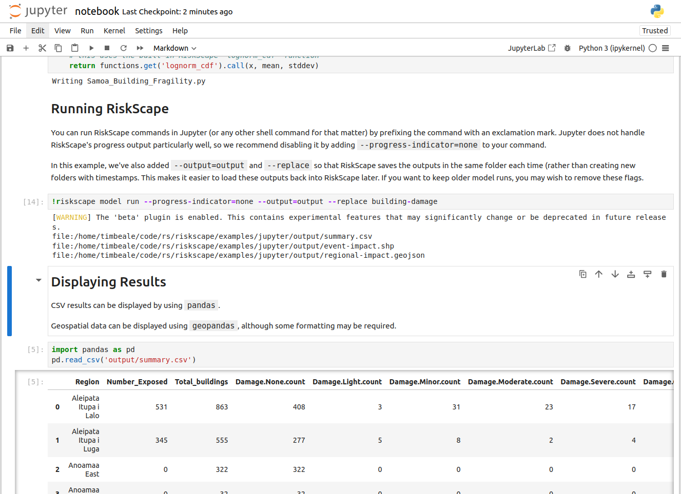
You can run RiskScape commands in Jupyter (or any other shell command for that matter) by prefixing the command with an
exclamation mark. Jupyter does not handle RiskScape’s progress output particularly well, so we recommend disabling it
by adding --progress-indicator=none to your command.
In this example, we’ve also added --output=output and --replace so that RiskScape saves the outputs in the same
folder each time (rather than creating new folders with timestamps). This makes it easier to load these outputs back
into RiskScape later. If you want to keep older model runs, you may wish to remove these flags.
!riskscape model run --progress-indicator=none --output=output --replace building-damage
Try playing the cell containing the riskscape model run command.
When RiskScape runs successfully, you should see the model result files displayed like this:

Note
Jupyter Notebook needs to be able to find the RiskScape executable on the PATH
environmental variable, in order for the RiskScape command to successfully run.
For Windows users, we typically recommend using a desktop shortcut to run RiskScape, which will
not permanently update the PATH. You can refer here for
how to set the PATH permanently on Windows (but be careful with this).
Or alternatively, you can use the full path to the RiskScape executable in the Jupyter
Notebook command, e.g. C:\RiskScape\riskscape\bin\riskscape model run ...
Visualizing results
Your RiskScape models can produce either tabular CSV results or geospatial outputs.
CSV results can be displayed simply by reading the data into pandas. The below will display a nice table of results.
import pandas as pd
pd.read_csv('output/summary.csv')
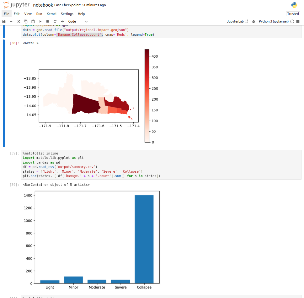
Geospatial data can be displayed using geopandas, although some formatting may be required.
%matplotlib inline
import geopandas as gpd
data = gpd.read_file("output/regional-impact.geojson")
data.plot(column='Damage.Collapse.count', cmap='Reds', legend=True)
You can also use matplotlib to visualize CSV or geospatial data,
for example producing bar or scatter graphs of the results.
For example, a bar graph breakdown of the total buildings in each damage state can be produced using:
%matplotlib inline
import matplotlib.pyplot as plt
import pandas as pd
df = pd.read_csv('output/summary.csv')
states = ['Light', 'Minor', 'Moderate', 'Severe', 'Collapse']
plt.bar(states, [ df['Damage.' + s + '.count'].sum() for s in states ])
Try playing the cells in the ‘Displaying Results’ section of your notebook now. You should see the model result files displayed like this:

Alternative way to run the model
As well as running a RiskScape model as shell command, you can also run a model directly from Python, like this:
import os
MODEL = 'building-damage'
os.system('riskscape model run --output=output --replace ' + MODEL)
This alternative approach can be handy if you want to loop over several model runs, or pass Python variables through as model parameters.