Geoprocessing your input data

Before we start

This tutorial is aimed at users who want to use RiskScape to model damage to larger elements-at-risk, such as roads. We expect that you:

• Have completed the Going beyond simple RiskScape models tutorial.

• Have a basic understanding of geospatial data and risk analysis.

• Have a GIS application (e.g. QGIS) installed that you can use to view shapefiles.

The aim of this tutorial is to explore the ways in which RiskScape can modify the geometry in your input data on the fly, so that you can build accurate loss models.

Getting started

Setup

Click here to download the example project we will use in this guide. Unzip the file into a new directory, e.g. C:\RiskScape_Projects\.

Open a command prompt and cd to the directory where you unzipped the files, e.g.

cd C:\RiskScape_Projects\geoprocessing-tutorial

You will use this command prompt to run the RiskScape commands in this tutorial.

The unzipped geoprocessing-tutorial\data sub-directory contains the input data files we will use in this tutorial. This data is similar to the Upolu tsunami data that we used in the previous tutorials, except that our exposure-layer is now a dataset of roads rather than buildings.

Note

This input data was provided by NIWA and is based on Open Street Map data for south-eastern Upolu. The regional map of Samoa was sourced from the PCRAFI (Pacific Risk Information System) website. The data files have been adapted slightly for this tutorial.

The geoprocessing-tutorial directory also contains a project.ini file that contains some pre-existing models we will use to demonstrate the various geoprocessing techniques.

Background

So far we have been using a building dataset for all our example models. Instead of modelling damage to buildings, if we were to model damage to roads it introduces some additional complexities:

• The element-at-risk is much larger. For example, a road may be many kilometres long and so some parts of the road may be completely unexposed to the hazard while others are severely damaged. It may be useful to cut the road into smaller segments and model the damage to each segment individually.

• Roading data is typically stored as line-string geometry, whereas in real-life the road may be several metres wide. You may want to enlarge the roads so they more realistically cover the area that will be exposed to the hazard.

• Working with larger, more complicated geometry is more computationally expensive and therefore your model may be slower to run. When you have a large dataset you can spatially filter the input data so that only elements-at-risk in the area of interest are run through the model.

RiskScape’s geoprocessing features allow us to modify the input data before it gets used in our model. We can cut long roads into 10-metre segments, enlarge them by a designated width so they become polygons, or filter our input data by the bounds of the hazard or a region of interest.

So far we have skipped over RiskScape’s geoprocessing functionality, but this tutorial will now look at the optional geoprocessing phase of the model workflow (shown below, click to enlarge the image) in more detail.

Note

This tutorial will focus on roads, but the same concepts apply to any large elements-at-risk, such as farmland, water pipes, or transmission lines.

Tip

We will focus on geoprocessing the exposure-layer, but RiskScape supports geoprocessing any vector layer (i.e. any shapefile data). For example, if your hazard-layer contained point data, you could buffer the points to turn them into larger polygon circles.

Cutting

How you handle large elements-at-risk, such as roads, depends somewhat on what you are trying to model.

Let’s start off with a simple model that tries to work out how much roading is exposed to the tsunami. Our input data already has a length (in metres) for each road segment, so we can try summing the lengths of all exposed road segments.

Run the following command in your command prompt:

riskscape model run simple-exposure

Note

You may notice that the models in this tutorial are slightly slower to run. This is because the road geometry is more complex than the simple building data we have been using so far. When the input data involves more complex geometry, or the hazard grid is smaller resolution, then the model’s processing will be more computationally expensive.

Running this model should produce an event-impact.csv results file that looks like the following:

Region,Exposed_segments,Exposed_km
Aleipata Itupa i Lalo,24,24.287
Aleipata Itupa i Luga,30,19.661
Falealili,67,42.263
Lepa,10,7.69
Lotofaga,41,16.58

The problem with this approach is that it overestimates how much road is exposed to the tsunami.

The road segments can be very long, but only a small area of road might be exposed to the tsunami. So counting the whole length of the road will over-represent the true clean-up or repair cost.

We will now look at a few different ways we can make our RiskScape model more accurate.

Cutting by distance

The simplest approach to deal with large elements-at-risk is to cut them into smaller segments. For example, instead of trying to model the damage to a 5km stretch of road, you could cut the road into smaller 10m segments and then model the damage to each segment individually.

RiskScape cuts geometry using the following approach:

• Line-string input geometry, such as roads, will be cut into segments of the specified length (or less, for the last segment).

• Polygon input geometry will be cut using a square grid. Each side of the grid will have the specified length. So cutting a polygon by a distance of 100m will result in 100m x 100m segments (10000m²) or smaller.

Tip

Line-strings can also be cut by a grid, rather than by length, but this is currently a pipeline feature. This lets you cut line-strings into pieces that exactly match the hazard grid.

For example, the following diagram shows how a block of farmland (grey outline) would be cut into segments that better correspond to the underlying hazard layer.

In this case we are dealing with road data, so we will cut them by length rather than grid. The project contains a cut-by-distance model, which will cut our roads into 50m segments, which is the same size as the hazard grid resolution.

Run the following command:

riskscape model run cut-by-distance

This should produce an event-impact.csv results file that looks like this:

Region,Exposed_segments,Exposed_km
Aleipata Itupa i Lalo,200,9.558
Aleipata Itupa i Luga,237,11.301
Falealili,347,15.936
Lepa,116,5.588
Lotofaga,108,4.138

You can see that the Exposed_segments values are much larger, because they are now dealing with smaller 50m segments. Whereas the Exposed_km values are much smaller because large parts of the original roads were not exposed to the hazard.

This model also saves the raw results after the geoprocessing has cut the exposure-layer, as a exposure-geoprocessed.shp output file. This lets you see exactly how RiskScape has modified your exposure-layer.

Open the exposure-geoprocessed.shp in QGIS, or your preferred GIS application. Use the ‘Identify Features’ tool (Ctrl+Shift+I) in QGIS and click on the road segments. You should see that each line-string is now no more than 50m long (i.e. the length attribute).

If you open the attribute table in QGIS, you will see that RiskScape has assigned each element-at-risk a SegmentID attribute. The SegmentID gets incremented for each segment cut from the same original line-string.

Recomputing attributes

When you cut an element-at-risk into smaller segments, you may also want to update its attributes to reflect its change in size. For example, your input data may contain attributes such as area, length, or repair_cost that will no longer be valid for the smaller segments.

The RiskScape wizard gives you two options after cutting your input data:

• Scale attributes: RiskScape can automatically adjust attributes based on the change in size. This can be useful for attributes such as repair cost. For example if a 1km road is cut into 10 segments, then RiskScape can adjust the repair_cost for each segment so that it is one-tenth the original value.

• Recompute attributes: For attributes such as area or length, it can be simpler just to recompute a new value for the attribute. For example, the cut-by-distance model replaced the input road’s length attribute by measuring the new length of the cut segment.

Tip

You can use the expression measure(exposure) to recompute the length of line-strings in your exposure-layer, or the area for polygon data. We will learn more about RiskScape expressions soon.

Alternatives to cutting

Instead of cutting the input data, you can use the aggregate by consequence functionality we covered in the Going beyond simple RiskScape models tutorial. It depends somewhat on what you want to model.

The all-intersections spatial sampling essentially already cuts the element-at-risk into segments that intersect with the hazard-layer. It also calculates an exposed_ratio attribute, which is the amount that each element-at-risk was exposed to the hazard.

This exposed_ratio attribute is typically used to scale the loss. However, we can also use the exposed_ratio here to calculate the total length of road exposed to the tsunami, i.e. exposed_ratio * exposure.length.

Try running the exposed-length model using the following command:

riskscape model run exposed-length

This should produces a raw-analysis.shp output file, which contains the intermediate results. This shapefile contains the exposure-layer geometry segmented by where it intersects the hazard-layer.

Note

Although the hazard-layer effectively has a 50m resolution, the pixel size in the GeoTIFF is actually 5m. So the roads are cut using a 5m grid here, rather than a 50m grid.

The command should also produce an event-impact.csv results file that looks like this:

Region,Exposed_segments,Exposed_km
Aleipata Itupa i Lalo,24,10.661
Aleipata Itupa i Luga,30,12.333
Falealili,67,14.088
Lepa,10,0.902
Lotofaga,41,5.489

Notice that the Exposed_km values are similar to the cut-by-distance model, except for the Lepa region which is quite different (0.9km vs 5.6km). This difference is because the Lepa road segments are large and are actually centred in the neighbouring regions, such as Lotofaga. The cut-by-distance cuts these roads into smaller segments which get assigned to the Lepa region. Whereas the exposed-length model matches the whole original road against the area-layer.

RiskScape has one more cutting feature that can help in this case.

Cutting by layer

Instead of cutting by distance, you can also cut your input data against geometry in another layer. For example, we can cut our roads by the regional boundaries in our area-layer.

The following diagram shows a simple example of how this works.

The cut-by-layer model works the same as the exposed-length model, except it cuts the roads along the area-layer boundaries before doing any other processing. Try running the model using the following command:

riskscape model run cut-by-layer

This should produce an event-impact.csv results file that looks like this:

Region,Exposed_segments,Exposed_km
Aleipata Itupa i Lalo,25,9.216
Aleipata Itupa i Luga,37,10.614
Falealili,68,14.799
Lepa,12,5.225
Lotofaga,42,3.62

The Exposed_km value for Lepa now looks more reasonable because the original roads were cut along the regional boundaries.

A exposure-geoprocessed.shp output file should also have been produced. Open this file in QGIS to see how RiskScape cut the input geometry.

Tip

You can optionally copy attributes from the cut-layer into your exposure-layer, such as the Region name. This can avoid having to specify a separate area-layer input, as it will typically be the same as the cut-layer.

Filtering

As you may have noticed, RiskScape models tend to run slower as they do more complex geometry processing. We can speed models up by using filtering to throw away input data that we are not interested in.

Filtering avoids unnecessary processing. For example, cutting can be computationally expensive. Therefore, cutting up input data that we will not use in our results can waste a lot of time.

There are three different ways you can filter your input data:

• by expression

• by a layer’s bounds

• by a feature in another layer, e.g. a region

Filter by expression

This approach checks whether an attribute in the input data satisfies a given condition before the data will be used in the model.

The following diagram is a simple illustration of filtering, where the squares represent input data attributes and the colours represent different values.

For example, if you were only interested in what bridges were exposed to the tsunami, then you could use the filter: exposure.bridge = 'T'.

Tip

The wizard will help you build these filter expressions interactively. This filtering is similar to the ‘Marine area’ bookmark filter in the project tutorial.

Filter by layer bounds

We will usually not be interested in elements-at-risk that fall outside the bounds of the hazard-layer, as we know they will not be impacted by the hazard at all. We can spatially filter our exposure-layer by the bounds of the hazard-layer to avoid unnecessarily processing these elements-at-risk.

The following diagram is a simple illustration of filtering out roads based on the bounds of flood inundation.

This filtering approach is useful when the exposure-layer dataset is wide-spread, but hazard is localized.

The exposure-layer data in this project has already been filtered by the bounds of the hazard to speed up running models. We know the tsunami hazard only impacts south-eastern Upolu, so cutting roads located on other islands of Samoa, such as Savai’i, would be unnecessary extra processing.

Note

Filtering by layer bounds can currently only be used when both input layers are in the same CRS.

Filter by region

Sometimes we might only be interested in the impact to a specific region.

The wizard reporting options let us filter the output results by region. However, this still means that a lot of unnecessary processing gets done for the other regions that we are ignoring.

RiskScape lets you filter your input data by a region of interest. For example, the following diagram is a simple illustration of filtering farmland based on a region of interest.

The filter-by-region model filters the input data so that only roads for the Falealili region are included in the model. Try running this model using the following command:

riskscape model run filter-by-region

This should produce a exposure-geoprocessed.shp output file, which shows the roads that will actually be used in the model. Open exposure-geoprocessed.shp in QGIS and take a look at it.

The command should also produce an event-impact.csv results file that looks like this:

Region,Exposed_segments,Exposed_km
Falealili,67,14.088
Lotofaga,1,1.328

Note

This filtering includes any input data that intersects the region of interest. Whereas matching against the area-layer uses the centroid of the road. So here the results include one road that is centred in the Lotofaga region, but still intersects the Falealili region.

As well as the Lotofaga road, there will also be other roads that extend into neighbouring regions. Let’s look at another example where we include only the roads that fall within the bounds of a given region.

Including only a region

Let’s say we want to only include the roads within the Falealili region in our model, and exclude any roading that falls outside that region.

To do this, we could combine several different approaches we have already learnt about:

• Filter the input data by the Falealili region.

• Cut by area-layer. This will cut any roads that ‘straddle’ regions into two.

• Filter results by the Falealili region again. This will remove any segments that fall into neighbouring regions.

However, we will now look at the include-only-region model which uses a slightly different approach. The cut-by-layer functionality can behave like the GIS ‘clip’ operation, in that RiskScape can throw away any geometry that falls outside the polygon(s) in the cut-layer.

For this to do work, we want the layer we are cutting against to only include the Falealili region polygon. We can add a simple bookmark with a filter statement that does this:

[bookmark Only_Falealili]
location = data/Samoa_constituencies.shp
filter = Region = 'Falealili'

When we cut against this Only_Falealili layer, it will cut all the roads at the Falealili boundary and throw away any parts of the original road that fall outside that region.

Try running this model using the following command:

riskscape model run include-only-region

This should produce an event-impact.csv results file that looks like this:

Region,Exposed_segments,Exposed_km
Falealili,68,14.799

This will also produce a exposure-geoprocessed.shp output file, which shows the roads after they have been ‘clipped’. Open exposure-geoprocessed.shp in QGIS and see how it differs compared to the filter-by-region shapefile.

Enlarging

The final geoprocessing feature we will look at is enlarging, or buffering. Buffering lets you enlarge polygons, or turn points or line-strings into polygons. The following diagram shows road line-strings that are buffered and turned into polygons.

Buffering can be useful when working with roading data. The road geometry typically only follows the centre-line, whereas the real-life road might be several metres wide. Enlarging the road line-string means that you detect hazards that intersect the road, but do not intersect the centre-line.

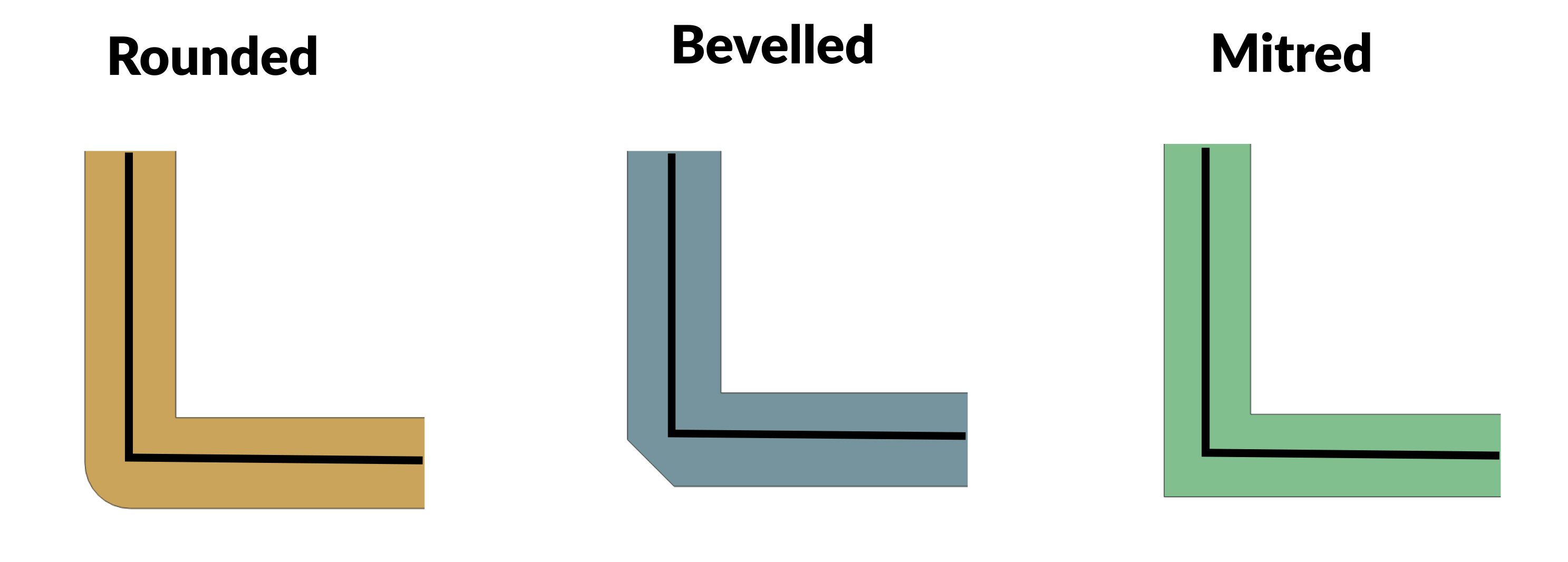
When you buffer shapes you have choices about what the enlarged shape will look like. For line-strings and polygons you can choose whether the corners should be rounded, bevelled, or mitred. The following diagram shows the difference between the approaches:

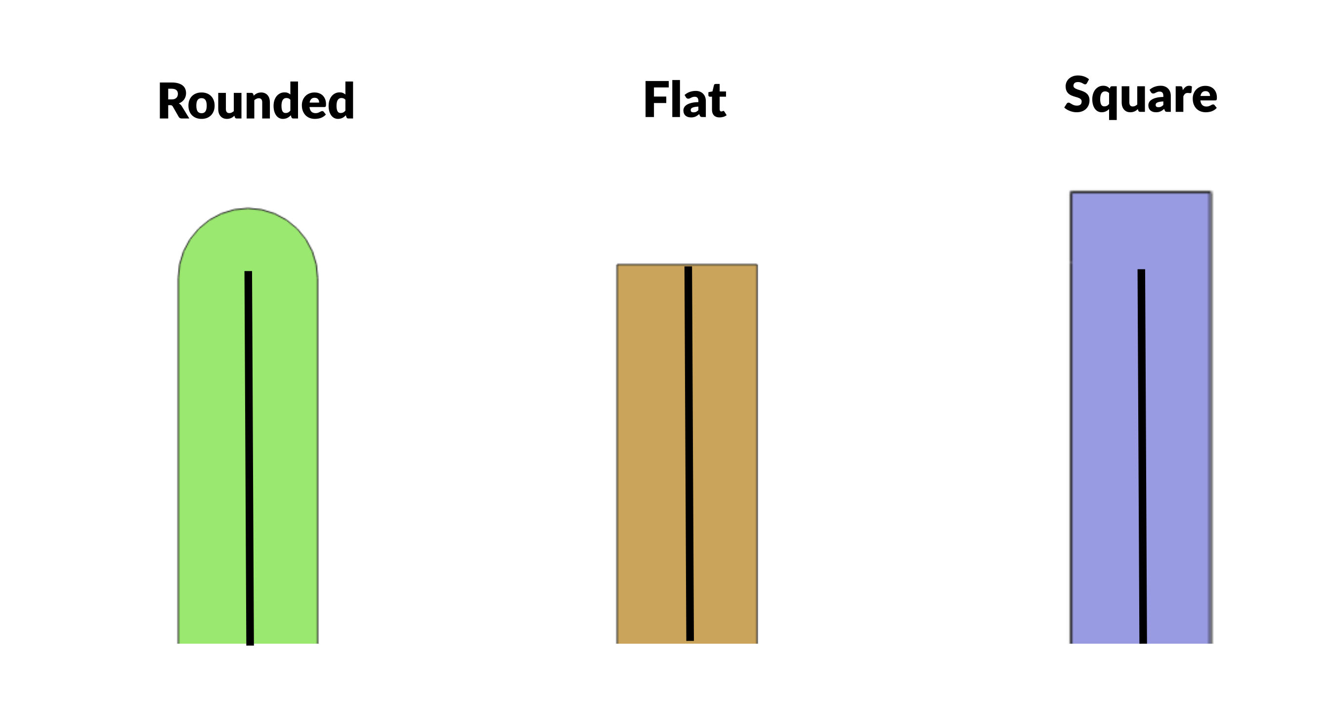
For line-strings, you can also choose whether the end of the line should be rounded, flat, or square. The following diagram shows the difference between the approaches.

Tip

When enlarging roads, we recommend using mitred corners and flat line-endings. This keeps the original shape of the line-string, but the road does not become any longer.

Buffering roads

Try running the buffer-roads model using the following command:

riskscape model run buffer-roads

This will produce a exposure-geoprocessed.shp output file, which shows what the roads look like after they have been buffered.

Note

This example data deals with a mixture of main highways, single-lane roads, and footpaths. So we have enlarged the road by a variable amount based on the type of road (its fclass attribute). You may simply choose to enlarge all roads by a constant, fixed distance.

In this model we calculate a width_metres attribute in the bookmark, based on the number of lanes that the road has. We then use half this value to buffer the road, i.e. exposure.width_metres / 2.

Tip

The line-string will be enlarged by the given distance in each direction. So the buffer distance should be half the total width of the road.

The model should also produce an event-impact.csv output file that looks like this:

Region,Exposed_segments,Exposed_km,Exposed_m2
Aleipata Itupa i Lalo,25,24.427,30515
Aleipata Itupa i Luga,30,19.661,32572
Falealili,67,42.263,36775
Lepa,10,7.69,2277
Lotofaga,41,16.58,11937

We have not cut the roads at all, and the buffered roads are now polygons rather than line-strings. So the Exposed_km is based on the original road-length, similar to the first simple-exposure model.

The hazard-layer here is a coarse 50-metre grid, and so buffering the road by a few metres has only detected one extra road as being exposed. However, the results now shows us how many square metres of road were exposed to the hazard.

Removing overlaps

In QGIS, if you zoom in closely to the buffered exposure-geoprocessed.shp file, you will notice that the buffered roads now overlap slightly at intersections.

These overlaps mean that the area impacted by the hazard can be counted multiple times at intersections. In a city grid with a lot of intersections, this double-counting could potentially over-represent the true damage from the hazard.

RiskScape has an option to remove these overlaps by cutting the buffered polygon. Overlaps are removed on a ‘best effort’ basis.

Try running the buffer-no-overlap model using the following command:

riskscape model run buffer-no-overlap

Open the resulting exposure-geoprocessed.shp output file in QGIS. This file looks similar to the previous buffer-roads model, except now if you zoom in to look at intersections you will see that the polygons have been cut so they do not overlap.

If you open the event-impact.csv output file, it should look like this:

Region,Exposed_segments,Exposed_km,Exposed_m2
Aleipata Itupa i Lalo,25,24.427,30452
Aleipata Itupa i Luga,30,19.661,32480
Falealili,67,42.263,36640
Lepa,10,7.69,2246
Lotofaga,41,16.58,11915

The Exposed_m2 values are now slightly lower compared with the buffer-roads model. However, as the tsunami impacts mostly coastal roads here, the total difference is only approximately 350 square metres.

Geoprocessing performance

RiskScape’s geoprocessing features let you alter your input geometry on the fly. This avoids cumbersome and potentially error-prone steps where you modify the data by hand.

However, you may have noticed that geoprocessing can add a performance overhead. In particular, cutting geometry into very small pieces, such as 1-2 metres, can be very slow and can greatly increase the memory (RAM) that running your model consumes.

If you want to run the model repeatedly, it can be quicker to save a copy of the geoprocessed data and use that file as the input to your model. This means RiskScape only needs to cut the data once.

Tip

You can save and run a model that only does geoprocessing. In the wizard, you can access the Ctrl + c menu part way through building your model, and that lets you save it.

Expressions

RiskScape uses its own expression language as the ‘glue’ that holds your model together. RiskScape expressions are simple statements that are similar to what you would use in a spreadsheet formula.

For example, to produce the Exposed_segments attribute in the results, we use the aggregate expression count(exposure) as Exposed_segments. The wizard will usually help you build these expressions, but there are limits to what you can do in the wizard. In order to do more advanced things in RiskScape, it is useful to be able to modify and write expressions yourself.

For example, you can use the wizard to build an expression like sum(exposure.length) as Exposed_metres. But converting this value to kilometres instead of metres is a slightly more complicated expression that you would have to enter manually, e.g. sum(exposure.length) / 1000 as Exposed_km.

Tip

In your project.ini file, you can edit the expressions in your saved model configuration manually. Writing your own expressions gives you more flexibility with your model than the wizard provides by default.

We will look at How to write RiskScape expressions in more detail in the next tutorial.

Recap

Let’s review some of the key points we have covered so far:

• Geoprocessing lets you modify your input geometry on-the-fly, in a deterministic way. You can cut large elements-at-risk into smaller segments, buffer them to enlarge the geometry, or spatially filter the input data to avoid unnecessary processing.

• RiskScape supports geoprocessing any vector layer in your model. Typically geoprocessing is useful for things like roads, water pipes, transmission lines, and farmland.

• Geoprocessing essentially creates a new exposure-layer that your model will use. Geoprocessing always takes effect before any other processing in your model, such as spatial sampling or consequence analysis.

• Cutting your input data lets you deal with large assets on a finer-grain level. You can either cut by a fixed distance or cut using geometry in another vector layer. However, cutting by a small distance can greatly increase your model’s memory usage and execution time.

• After cutting your exposure-layer, you may need to adjust attributes to reflect the change in size, i.e. area, length, repair_cost, etc. You can either automatically scale the attributes by the amount they have decreased in size, or recompute the values from scratch.

• Filtering lets you remove input data that you are not interested in from your model. Excluding input data means your model will run quicker. This can be useful when you have a large exposure-layer dataset, but a small area of interest.

• Buffering or enlarging will increase the area of each element-at-risk. This can mean that road line-strings are more realistically spatially matched against the hazard-layer. Buffering will turn line-strings into polygons.

• To do more complicated things in your models it is useful to be able to modify RiskScape expressions.

Extra for experts

If you want to explore the concepts we have covered a little further, try using the riskscape wizard command to build your own geoprocessing models.

• Tip: Focus on the geoprocessing side of things. Select the option to ‘Save the modified layer after the geoprocessing has taken effect’ so you can see what the geoprocessing does. For simplicity, just use the ‘closest’ spatial sampling, and filter the results based on consequence = 1 (i.e. only include the exposed road segments in the results).

• Try creating models that:

  • Cut the roads by a fixed distance, e.g. 10m.

  • Filter the road input data by the Lepa region.

  • Enlarge all the roads by 3 metres in either direction.

• Try running the cut-by-distance model with a different cut-distance, i.e. -p "input-exposures.cut-distance=5". Try it with 5 metres and then again with 100 metres. Pay attention to how long the model takes to run each time.