How to build RiskScape models
Before we start
This tutorial is aimed at new users who want to start building their own risk models in RiskScape. We expect that you:
Have completed the Getting started modelling in RiskScape guide and are familiar with running a RiskScape model from the command-line.
Have a basic understanding of geospatial data and risk analysis.
Have GIS software (e.g. QGIS) installed that you can use to view shapefile and GeoTIFF files.
Note
ArcGIS users should read Workarounds for ArcGIS before proceeding. It lists tips to ensure that geospatial data is projected correctly in ArcGIS.
The aim of this tutorial is to get you familiar with using the CLI wizard so you can start building your own models.
For simplicity, this tutorial will not delve into much detail around creating bookmarks, writing your own functions, or writing pipelines from scratch. These topics will all be covered in later tutorials.
Getting started
Setup
Click here to download the example project we will use in this guide.
Unzip the file into the Top-level Windows project directory where you keep your RiskScape projects.
For example, if your top-level projects directory is C:\Users\%USERNAME%\RiskScape\Projects\,
then your unzipped directory will be:
C:\Users\%USERNAME%\RiskScape\Projects\wizard-models
Open a command prompt and cd to the directory where you unzipped the files, e.g.
cd wizard-models
You will use this command prompt to run the RiskScape commands in this tutorial.
The input data files this tutorial will use are all in the wizard-models\data sub-directory.
This is similar to the Upolu tsunami data that we used in the previous tutorial,
except that for simplicity, our building database now uses centroid points instead of polygon geometry.
Note
This input data was provided by NIWA, as well as the PCRAFI (Pacific Risk Information System) website. The data files have been adapted slightly for this tutorial.
Alongside the data sub-directory, there is a project.ini file in your unzipped directory.
This file contains some pre-existing bookmarks and functions, which you will use to build models in the wizard.
Model workflow
The processing workflow for a RiskScape model is split up into phases, which are shown in the following diagram:
The grey boxes denote the model phases. We will look at each phase of the model workflow in more detail, as we go along.
The navy-coloured boxes illustrate the inputs that you provide the model with. You supply RiskScape with the input data files that the model will use, and the function that will analyse the impact that the hazard has on each element-at-risk.
You also need to give RiskScape instructions on how it should process the data for each phase in the model workflow. The wizard will ask you a series of questions in order to gather all the information it needs to build a model.
Building a simple exposure model
We will now walk-through the process of building a simple exposure model in the wizard. We will take our Upolu building dataset and identify what buildings are exposed to tsunami inundation, based on the 2009 South Pacific Tsunami (SPT) event.
Running the wizard
To start the wizard, simply enter the following command into your terminal prompt:
riskscape wizard
Tip
Make sure you run the wizard command from the directory that contains your project.ini file,
as this file tells RiskScape where to find your input data and functions.
In this case, the directory you unzipped contains a project.ini file that we have
already created for you.
When you first run the wizard, it will print out a blurb that outlines the phases in the model workflow:
riskscape wizard
RiskScape™ Copyright Institute of Geological and Nuclear Sciences Limited
& National Institute of Water and Atmospheric Research Limited is distributed
for research purposes only under the terms of AGPLv3.

This wizard will guide you through the questions required to build a risk model.
The following sets of questions will be covered:
 - input-data: Specify the input data sources for your risk model
 - geoprocess: Optionally modify each vector layer before it gets used by the model
 - sample: Specify how to spatially match up each element at risk against the hazard-layer
 - analysis: How to determine the consequences that the hazard has on the exposure-layer
 - event-impact-report: Change how the final event impact results are presented and saved to file
 - reports: Add another output file to your model
 Use ctrl-c to see a help menu at any time
We will now walk-through the questions that the wizard asks you, one phase at a time.
Tip
You can press Ctrl and c at any time to see a wizard menu with additional options.
We won’t need to use most of these options in this tutorial, but there is an ‘Undo’ option available
if you enter an incorrect answer in the wizard and want to go back and change it.
Input data phase
The first prompt we get is the following, which relates to the input data layers that your model will use.
Choose a set of questions to answer next

1:  Choose and configure exposures layer
2:  Choose and configure hazards layer
3:  Choose and configure first hazard layer (Multi-Hazard)
4:  Choose and configure areas layer
5:  Choose and configure resources layer
You may recall from the previous tutorial that a RiskScape model has the following layers:
- Exposure-layer
This contains the elements-at-risk that are potentially impacted by the hazard. For example, these may be building, roads, infrastructure, or even population density or land-use maps.
- Hazard-layer
This contains the geospatial footprint of the hazard you are modelling.
- Area-layer
This contains regional boundaries that can optionally be used to collate the results. For example, if you wanted a breakdown of damage or losses by district or region.
- Resource-layer
This contains any supplementary geospatial data that may be needed by your model. For example, if you are modelling an earthquake then you may need to know the soil-type underneath a building in order to calculate liquefaction damage.
Let’s start by picking the exposure-layer for our model.
Simply type the number of the option you wish to choose (i.e. 1) and press enter.
The wizard will then present us with options for the next question, which will look like the following:
input-exposures >> layer

Choose an exposure layer. This contains the elements at risk (e.g. buildings, roads) that will
be exposed to the hazard layer(s).

1:  Building centroids SE Upolu (exposure-layer)
2:  SPT inundation 50m grid (hazard-layer)
3:  Samoa constituencies (area-layer)
These options are the bookmarks in our project. A bookmarked data source is how we tell RiskScape about an input file to use in our model.
Note
Bookmarks get defined in your project.ini file.
We have provided you with a project.ini file that already has some bookmarks setup.
We want our exposure-layer to be the buildings database, so pick the first option (1).
The next choice the wizard presents us with looks like this:
input-exposures >> geoprocess

Do you want to modify this input data at all before it gets used by your model?

Geo-processing lets you filter out rows of data, enlarge geometry (such as points or lines),
or cut large geometry into smaller segments. Do you want to geo-process your exposures-layer
at all?

1:  yes
2:  no
Geoprocessing lets us manipulate the input geometry before it gets used in the model.
We will look at RiskScape’s geoprocessing options more in a later tutorial,
so just answer ‘no’ for now. Type either 2 or n and press enter.
RiskScape will now give you the option of specifying the other layers that your model will use:
Choose a set of questions to answer next

1:  Choose and configure hazards layer
2:  Choose and configure first hazard layer (Multi-Hazard)
3:  Choose and configure areas layer
4:  Choose and configure resources layer
Enter 1 to choose a hazard-layer.
RiskScape will give us a list of the project’s bookmarked data sources again.
This time, enter 2 to pick the SPT inundation 50m grid (hazard-layer) bookmark.
Note
We are not offered a follow-up geoprocessing question this time. This is because the hazard-layer is raster data (a GeoTIFF), and RiskScape only supports geoprocessing for vector data, such as shapefiles.
RiskScape will then ask us if there are any other optional layers we would like to add, i.e.
Choose a set of questions to answer next

1:  Choose and configure areas layer
2:  Choose and configure resources layer
3:  skip
Enter 3 to skip and to move on to the next phase of the model workflow.
Spatial sampling phase
Once we have entered our input data, RiskScape presents us with the next phase of the model workflow:
Choose a set of questions to answer next

1:  Sampling Phase:  Specify how to spatially match each exposure-layer element against the other layer(s)
In the Spatial Sampling phase, RiskScape geospatially combines the input layers in your model. For example, it spatially matches each element-at-risk against the hazard-layer in order to determine the hazard intensity measure (if any) that affects it.
You could think of sampling as being like putting a pin into a map and plucking out the data at the point where it lands. In this case, we have the centroid of a building footprint, and we are plucking out the inundation depth at that point. Conceptually, it looks something like this:

Type 1 and press enter to start answering the Spatial Sampling questions.
RiskScape will present us with a choice of spatial matching techniques:
How do you want to spatially match each exposure-layer element against your hazards-layer?

How you detect spatial matches between the exposure-layer and the hazards-layer may depend somewhat on what
you are modelling. Pick the option that best suits your input data.

1:  centroid:   Use the centroid point of the element-at-risk's geometry to find a match in the other layer.
                This is a very predictable approach, but may miss cases where the layers do intersect but just
                not at the centroid.
2:  closest:    Look for anywhere the element-at-risk's geometry intersects with the other layer. If multiple
                matches are found then the one that is closest to the exposure's centroid is chosen. This is a
                good all-round approach, and a buffer/margin-of-error can also be applied when looking for
                matches.
We will learn more about how the different spatial matching techniques work in a subsequent tutorial.
The building data geometry that we are using here consists of centroid points, so we can simply choose ‘centroid’ sampling.
Type 1 and press enter.
Tip
The ‘closest’ sampling is generally a good default choice for most models, as it works well for lines and polygons, as well as points. We use ‘centroid’ sampling in these examples purely for simplicity.
Consequence analysis phase
The next phase of the model workflow is the Consequence Analysis phase:
Choose a set of questions to answer next

1:  Analysis Phase:  How to determine the consequences that the hazard has on the exposure-layer
In this phase, RiskScape applies a Python function to every element-at-risk in your exposure-layer, using the hazard intensity measure that was determined by the sampling phase. This function will calculate the impact, or consequence, that the hazard has on each building.
Type 1 and press enter to start answering the Consequence Analysis questions.
RiskScape presents us with a list of functions we can potentially use for our model.
Select a function to determine the consequence the hazard has on each exposure-layer element.

Please specify a function to evaluate each element-at-risk and hazard-intensity-measure and
produce a consequence.

1:  exposure_risk
2:  is_exposed
Note
Functions get defined in your project.ini file.
We have provided you with a project.ini file that already has a function setup.
You will learn more about adding your own functions in a subsequent tutorial.
The is_exposed function is a built-in RiskScape function that can be used in any exposure model.
The is_exposed function produces a consequence of ‘1’ if the element-at-risk was exposed to the hazard,
and ‘0’ if not.
Type 2 to select the is_exposed function and press enter.
Results reporting phase
The last phase of the model workflow is the Results Reporting phase:
Choose a set of questions to answer next

1:  Change how the final 'event-impact' results are presented and saved to file
2:  skip
This phase lets us customize how the model results are saved to file.
For now, we are going to skip this phase and come back to it later.
Type 2 and press enter.
Saving the model
We have now gone through all the phases in the model workflow. RiskScape now gives us the option of saving the model:
*** There are no further questions to answer. What do you want to do with your completed model? ***

1:  Save and run
2:  Save and quit (without running it)
3:  Run it (without saving it)
For new users, we recommend always selecting the first option, ‘Save and run’.
Type 1 and press enter.
RiskScape will then ask you for a name to save the model as.
Enter a name for the new model
>
If we want to re-run our model again later, this name will be used in the riskscape model run command.
Let’s call our model simple-exposure. Type that name in and press enter.
Note
At this point, we are just saving the instructions or the ‘blueprint’ for the model,
rather than the actual results from running the model.
The answers we entered in the wizard will now become the parameters for the saved model.
These model parameters get saved in a models_simple-exposure.ini INI file.
RiskScape will display the file path of your saved model.
You should then see output that is similar to using the riskscape model run command in the previous tutorial.
You may notice that RiskScape also saved a pipeline_simple-exposure.txt file.
This file represents the model workflow in a RiskScape-specific pipeline language.
Pipelines are an advanced concept that we will learn more about later.
Examining the results
The Consequence Analysis phase in the model workflow always produces an Event-Impact Table, which contains the results from our model.
After you saved your model, RiskScape should have ran the model and produced an event_impact_table.shp results file.
The RiskScape wizard saves its results to an output/wizard/<timestamp>/ sub-directory within the current working directory,
e.g. ./output/wizard/2022-01-12T14_26_48/event_impact_table.shp.
Open this event_impact_table.shp file in QGIS.
Tip
From the terminal you can enter the command qgis PATH_TO_SHAPEFILE to open a shapefile in QGIS,
e.g. qgis output/wizard/2022-01-12T14_26_48/event_impact_table.shp
At first glance, the file looks the same as the exposure-layer input data we started with. In QGIS, right-click on the layer and select ‘Open Attribute Table’. Let’s examine this data in more detail.
Event Impact Table
You can think of the data in a RiskScape model as being a bit like a big spreadsheet - each row of data represents an element-at-risk, and the columns represent attributes associated with the element-at-risk. As the input data moves through the model, the rows and columns can change.
For example, Spatial Sampling phase adds a hazard attribute to exposure-layer input data,
as shown in this simple example:
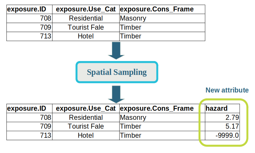
By the time the event-impact table is produced, the following attributes are always present in the data:
exposureThe data representing each element-at-risk, which corresponds to our exposure-layer input data. In this case, our exposure-layer containsID,Use_Cat, andCons_Frameattributes, as well as the geometry used in the shapefile.hazardThe hazard intensity measure that affected the element-at-risk, which is determined during the Spatial Sampling phase. In this case, it is the tsunami inundation depth, in metres. (Note that the shapefile uses the value-9999.0to represent ‘no data’, i.e. a building that was not exposed).consequenceThe impact or outcome that the hazard had on the element-at-risk. This is the return-value from the function used in the Consequence Analysis phase. In this case, the consequence is1if the building was exposed and0if not.
Note
The attribute names in a shapefile will always be truncated so that they are no more than 10 characters long,
so we end up with consequenc rather than consequence.
If a model has either of the optional area-layer or resource-layers specified,
then these would also appear in the Event Impact Table as area and resource respectively.
Re-running models
Once you have built a model in the wizard, you will probably want to re-run the model again later. For example, you may want to change some of the model’s parameters, such as the hazard-layer that it uses.
Enter the following command to see what models are available to run.
riskscape model list
In the output, you should see the simple-exposure model ‘blueprint’ that you saved earlier in the wizard.
Tip
When the auto-import setting is enabled in the project.ini file, RiskScape will automatically
try to load any wizard models that you save, i.e. the new models_simple-exposure.ini INI file.
The project.ini file we are using here has this setting enabled.
By default, the event-impact table gets saved as a shapefile because it has geometry present. Run the following command to save the model results as a CSV (Comma-Separated Values) file instead.
riskscape model run simple-exposure --format csv
Open the event_impact_table.csv file that was produced.
It should look something like this:
exposure.the_geom,exposure.ID,exposure.Use_Cat,exposure.Cons_Frame,hazard,consequence
POINT (422204.39138965635 8450380.92939743),1362,Outbuilding,Masonry,,0
POINT (422190.56381308025 8450230.231519686),1610,Residential,Masonry,,0
...
Note
The full attribute names now get saved in the CSV file.
For example, the exposure-layer Cons_Frame attribute now gets saved as exposure.Cons_Frame.
Bear in mind that the attribute names that appear in shapefile results files may be slightly
different to the attribute name used within the RiskScape model.
This is due to the 10-character limit that the shapefile format enforces.
Also note that the exposure-layer geometry (i.e. the exposure.the_geom attribute) gets saved as Well-Known Text (WKT) in the CSV file.
Building a model with regional aggregation
We will now use the wizard to build a slightly more complicated model that does the following:
Includes an area-layer so that we can aggregate the results by region.
Uses a simple Python function to determine the consequence.
Customizes how we report the Event Impact Table to use aggregation, i.e. report a total count of exposed buildings, instead of reporting every single exposed building.
Enter the following command to start the wizard again:
riskscape wizard
Input data phase
In the wizard, select the same exposure-layer and hazard-layer as you did previously, i.e.
Enter
1to choose the exposure-layer.Enter
1to select theBuilding centroids SE Upolu (exposure-layer)data.Enter
nto skip geoprocessing.Enter
1to choose the hazard-layer.Enter
2to select theSPT inundation 50m grid (hazard-layer)data.
Tip
Remember if you enter the wrong answer at any point in the wizard,
you can go back and change your answer. Simply press Ctrl and c
and select the ‘Undo’ option from the menu.
This time, we will also add an area-layer to our model. In the wizard:
Enter
1to choose an area-layer.Enter
3to select theSamoa constituencies (area-layer)data.Enter
nto skip geoprocessing.Enter
2to skip adding a resource-layer.
Spatial sampling phase
Again, we will use the same sampling answers as we did in our previous model. In the wizard:
Enter
1to select the Sampling Phase set of questions.Enter
1to use ‘centroid’ sampling.
You will now be presented with an extra optional question about the area-layer, i.e.
*** Pick A Question ***

1:  Specify a buffer (i.e. margin of error) when matching exposure-layer elements against the areas-layer
2:  Skip
This ‘buffer’ option is useful when some of our elements-at-risk fall just outside the area-layer boundaries.
This can be a particular problem in coastal areas, for example with ports or lighthouses that are actually located in the sea.
Enter 2 to skip this option for now.
Note
When you change an answer to a wizard question, it can ‘unlock’ more follow-up questions. For example, when we specified an area-layer as input data, the wizard then presented us with an additional follow-up spatial sampling question we could answer.
Consequence analysis phase
This time we will use our own Python function to analyse how each building is exposed to the tsunami inundation.
The project contains the following simple Python function, called exposure_risk,
which assigns each building into a risk category based on the level of inundation it is exposed to.
def function(building, hazard):
    if hazard is None or hazard == 0:
        return 'None'
    elif hazard <= 0.2:
        return 'Low'
    elif hazard <= 0.5:
        return 'Medium'
    else:
        return 'High'
Warning
This function is purely for demonstrative purposes and is not based on scientific methodology in any way.
RiskScape will pass our function two values: building and hazard.
We call these the function’s arguments.
The building argument represents a single row or record of data from our exposure-layer (which is our building database).
The hazard argument is a floating point number that we have sampled from the hazard-layer, i.e. it is the tsunami
inundation depth, if any, that is located at the centroid of the building.
The function’s return value will be added to the model’s results as the consequence attribute.
Now, in the wizard:
Enter
1to select the Analysis Phase set of questions.Enter
1to select theexposure_riskfunction.
Results reporting phase
We will now look at changing how we report the results from the model. Select 1 at the following prompt:
Choose a set of questions to answer next

1:  Change how the final 'event-impact' results are presented and saved to file
2:  skip
RiskScape then gives us the following range of operations that we can apply to the Event Impact Table data before it is saved to file.
*** Pick A Question ***

1:  Filter the output so that only certain results are included
2:  Aggregate the results, e.g. take the sum, count, mean, etc
3:  Select and adjust the columns/attributes included in the output
4:  Sort output by particular attribute(s)
5:  Specify the output file format (csv, shapefile, etc)
6:  Skip
These are all just different ways to manipulate the results data:
Filtering lets us exclude or include certain results, based on a given condition. For example, we could just report the buildings we have identified as being high risk.
Aggregating lets us summarize or collate the results. This is similar to spreadsheet operations like
COUNT()orSUM()that you would use across rows of data.Selecting lets us adjust or rename what attributes appear in the results file. For example, we could rename the
consequenceattribute toRiskto better suit our model.Sorting lets you order the results. For example, we could order the results by the
hazardattribute, so we can easily identify the buildings that are worst impacted by inundation.Finally, we can also specify the file format that the results get saved in.
We want to aggregate our results by region, so enter 2 in the wizard.
Aggregation
There are two parts to aggregation:
Grouping the results by the attribute(s) that we are interested in. This is how we want to see the model results broken down, such as by region or by building construction material.
Applying an aggregate function, such as
sum()orcount(), to each group of results. This is what collated result we want to see, such as the total count of affected buildings or the total monetary loss.
The wizard can also optionally aggregate your data into buckets, or bins. We will cover this in more detail later.
As a simple example, let’s say that our model produces a loss consequence, in dollars,
and we want to see the total losses broken down by the building construction material:
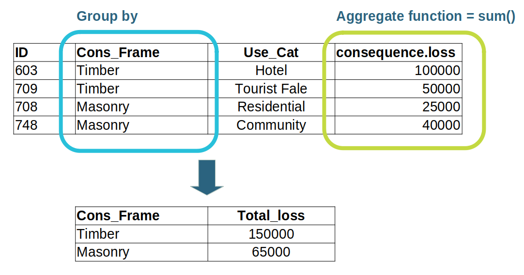
In this example, the building data is grouped based on the Cons_Frame attribute,
which means buildings that share the same construction material are grouped together.
We then use the sum() aggregate function to add together the loss values for all the buildings
that share the same construction material, and produce a Total_loss result.
Group by
In the wizard, RiskScape presents us with the first choice, of how to group the results:
Aggregate the results, e.g. take the sum, count, mean, etc

Specify the attribute(s) that the aggregated results should be grouped by. This is how you
want the results categorized, e.g. by area.name or exposure.construction.
Choose the attribute to use:

1:  exposure.the_geom
2:  exposure.ID
3:  exposure.Use_Cat
4:  exposure.Cons_Frame
5:  exposure
6:  hazard
7:  area.the_geom
8:  area.fid
9:  area.NAME_1
10:  area.Region
11:  area
12:  consequence
These are all the attributes that are currently in our Event Impact Table.
Note that the exposure and area data are Structs, which is a RiskScape term for a collection of attributes.
The exposure struct contains all the attributes that were present in the exposure-layer input data,
which in this case are ID, Use_Cat, and Cons_Frame.
The area struct holds all the area-layer input data attributes, which are fid, NAME_1, and Region.
In this case, we want to group the results by region (area.Region) and by the High/Medium/Low risk category
(which is the consequence that our Python function produced).
This means that any rows of data that have the same region and the same risk category will be grouped together.
In the wizard:
Enter
10to group byarea.Region.RiskScape will ask whether you want to rename the attribute. Enter
n.RiskScape will ask whether you want to give another response. Enter
y.Enter
12to also group byconsequence.Enter
nto skip renaming it.Enter
nto finish giving responses for the group-by question.
You will be asked to pick how you would like to aggregate the results. You can choose either Simple aggregation,
or Aggregate by buckets. If you choose Simple aggregation, you will be given the chance to apply bucket aggregation
later. If you choose to Skip, your data will not be aggregated, and the output will be all the groups generated by
the group by step. For example, if you grouped by region, you would get a list of all the regions in the input data.
For now, enter 1 to do simple aggregation.
Applying an aggregate function
RiskScape will then ask you what aggregation you want to apply to the grouped data:
Now specify which attribute values from the raw results you want to aggregate.

This is the attribute you want to see the total/max/average values for, e.g. consequence.loss, hazard.
Choose the attribute to use:

1:  exposure.ID
2:  hazard
3:  area.fid
In this case we simply want to count the total number of buildings in each group, so it doesn’t matter too much which attribute we pick.
Let’s use exposure.ID - enter 1 in the wizard.
Next, RiskScape asks you which aggregate function you want to use:
Specify how you want to aggregate this value.

Pick the aggregate function that will produce the result you're interested in.

1:  count
2:  max
3:  mean
4:  median
5:  min
6:  mode
7:  percentile
8:  percentiles
9:  stddev
10:  sum
Enter 1 in the wizard to use the count function.
Tip
Using a RiskScape aggregate function is conceptually similar to using a spreadsheet formula, like SUM(A1:A20),
where you have a function and a range of spreadsheet cells it applies to.
Picking the attribute to aggregate is like specifying the spreadsheet column in the formula.
Picking the attribute to group the data by determines which spreadsheet rows get collated together.
Finally, we need to give the aggregated result a name:
Specify a new name for the aggregated result.

This is the name that will be used for this value in the output results file.
>
Type Total_buildings for the new name and press enter.
Type n when asked to give another response.
Type 2 to Skip bucket aggregation.
Sorting the results
When we aggregate by region like this, it can be nice to sort the results file alphabetically based on the region’s name.
You should now have the following wizard prompt, which lets you choose from the remaining reporting operations.
*** Pick A Question ***

1:  Select and adjust the columns/attributes included in the output
2:  Sort output by particular attribute(s)
3:  Specify the output file format (csv, shapefile, etc)
4:  Skip
In the wizard:
Enter
2to sort the model’s results.Enter
1to sort on theRegionattribute.Enter
1to sort by ascending/alphabetical order.Enter
nto skip sorting on any other attributes.
Save and run the model
In the wizard, skip the remaining questions and save the model:
Enter
2to skip the remaining reporting option.Enter
2to skip adding a second output file.Enter
1to save and run the model. Call the modelrisk-by-region.
Once the model has run, it should produce an event-impact.csv file that looks something like the following:
Region,consequence,Total_buildings
,High,10
,None,4
Aleipata Itupa i Lalo,High,457
Aleipata Itupa i Lalo,None,340
Aleipata Itupa i Lalo,Medium,17
Aleipata Itupa i Lalo,Low,42
Aleipata Itupa i Luga,Low,31
Aleipata Itupa i Luga,None,221
Aleipata Itupa i Luga,Medium,26
Aleipata Itupa i Luga,High,272
Anoamaa East,None,322
Anoamaa West,None,32
Falealili,Medium,62
Falealili,Low,59
Falealili,None,1039
Falealili,High,602
Lepa,None,244
Lepa,Medium,11
Lepa,Low,20
Lepa,High,245
Lotofaga,Medium,11
Lotofaga,Low,19
Lotofaga,None,282
Lotofaga,High,111
Safata,None,595
Siumu,None,681
Vaa o Fonoti,None,404
Vaimauga West,None,101
Note
The Region field is blank for the first 2 entries in the results. This means that there were some buildings that fell outside any regional boundary in our area-layer.
Re-running the model
Your new risk-by-region model should now appear when you run the following command:
riskscape model list
Let’s try re-running our model, but this time in the Spatial Sampling phase we will use a buffer, or margin of error, when geospatially matching against the area-layer. Applying a buffer means that RiskScape actually enlarges the building’s geometry, if needed, so that it is more likely to spatially intersect the area-layer.
We chose to skip the sample.areas-buffer question in the wizard, but we can supply an answer to the question now as a model parameter.
Tip
Remember that when you run a model, you can specify additional model parameters by using the --parameter or -p
CLI option. You specify the parameter’s value in the format -p "PARAMETER_NAME=VALUE".
The parameters that a model uses are listed in the riskscape model list command output.
The buffer distance is in metres, so 1000 will match each building against the closest regional boundary, within a 1km radius.
Enter the following command in your terminal:
riskscape model run risk-by-region -p "sample.areas-buffer=1000"
Now check the event-impact.csv file that was produced.
You should notice that the entries with the blank Region attribute are no longer present.
Editing saved models
Using the -p CLI option when you run a model can be handy to try out one-off changes.
However, it gets a bit cumbersome if you have a lot of -p options you need to change.
As well as changing the model’s parameters on the CLI, you can also edit the parameters manually in the model’s INI file definition.
Open the models_risk-by-region.ini file in Notepad (or your preferred text editor).
Add the line sample.areas-buffer = 1000 to the bottom of the file and save it.
Enter the following command in your terminal to run the updated model:
riskscape model run risk-by-region
Check the event-impact.csv file that was produced.
You should notice that there are no blank Region entries still, even though we are no longer using the -p CLI option.
Recap
Let’s review some of the key points we have covered so far:
The wizard is structured around a conceptual model workflow, which is broken up into different phases: Input data, Geoprocessing (optional), Spatial Sampling, Consequence Analysis, and Results Reporting.
Each phase of the model workflow manipulates the input data slightly. This culminates in producing an Event Impact Table, which contains the consequence that the hazard had on each element-at-risk.
You can think of the model’s data as a bit like a spreadsheet. Each row of data represents an element-at-risk from the exposure-layer. Each column of data represents an attribute value, such as the hazard intensity measure (i.e. the
hazardattribute), or theconsequencethat the hazard has on the element-at-risk.The wizard uses bookmarks (for input data) and functions that have been setup in your
project.inifile.Depending on what answer you provide to a wizard question, it can ‘unlock’ more follow-up questions.
Saving a wizard model saves the ‘blueprint’ for the model, which means you can re-run the model again later (using the
riskscape model runcommand).The model’s parameters correspond to answers you gave to wizard questions. When you run a model, you can vary the model parameters, such as we did for
sample.areas-buffer. This can be a handy way to change what input layers your model uses.You can change the model’s parameters either by using the
-pCLI option, or by modifying the model’s INI file.The Results Reporting phase lets you customize how the Event Impact Table gets saved to file.
Aggregation lets you collate or summarize the Event Impact Table results. Aggregation groups together rows of data that have an identical attribute (e.g. region name), and then applies an aggregate function, such as
count(),sum(), ormean(), to attributes in the grouped results.
Once you feel comfortable using the wizard, you could try the next tutorial on Creating a RiskScape project.
Extra for experts
If you want to explore using the wizard a little further, you could try the following exercises out on your own.
Start building a new model in the wizard and then intentionally answer a question incorrectly. Press
Ctrlandcsimultaneously to bring up the wizard menu and undo your last answer.Run the
simple-exposuremodel, but this time change the Consequence Analysis phase to use theexposure_riskfunction, i.e. use-p "analysis.function=exposure_risk". Open the results file and see what effect this has on theconsequenceattribute.In the
exposure_risk.pyfile, try modifying the depths (i.e. 0.2m, 0.5m) that the risk categories use. Use values that you feel are more appropriate. Re-run therisk-by-regionmodel and see what difference your changes make to the results.In the
exposure_risk.pyfile, try adding aelifstatement that returns a new risk category, e.g. ‘Extreme’. Re-run therisk-by-regionmodel and see what difference this change makes to the results.Build the first model (i.e.
simple-exposure) in the wizard again, but this time customize the event-impact report at the end:Try adding a filter so that only the exposed buildings are included in the model’s results. Hint: the
consequenceattribute equals1when the building is exposed.Try using the ‘select’ reporting option to change the attribute/column names.
Select
exposure.the_geom, without renaming it.Select
hazardand rename it todepth.
Save your model, and then open the shapefile it produces in QGIS. Look at the attribute table and compare it to the results you got earlier.
The geometry in our exposure-layer is centroid points, whereas real life buildings typically have larger footprints. Try using a spatial sampling buffer with the hazard layer, so we look for tsunami inundation within 3 metres of the centroid point. Re-run the
risk-by-regionmodel with the parameters-p "sample.hazards-by=CLOSEST"and-p "sample.hazards-buffer=3". Check the results file that gets produced and see if this changes the number of buildings exposed to inundation.Open your
project.inifile in Notepad. Change theauto-importsetting tofalseand see what happens to your saved models, i.e.riskscape model list. Add amodels = models_simple-exposure.iniline to the[project]section to import a model manually. See what effect this has.Try using the aggregate by buckets option. After selecting the attribute(s) you would like to group by, choose
Aggregate by buckets. You will be prompted for:The attribute you’d like to use to divide the results into buckets. The ranges that you enter in the next question will be checked against this attribute.
The ranges or boundaries of the buckets. RiskScape will infer the two “end” buckets, e.g., if you input
1, then2, you will get four buckets: <1, 1-2, and >2The aggregation expression that will be evaluated for each bucket. This works the same as it does for simple aggregation.