Getting started modelling in RiskScape
Before we start
This tutorial is aimed at new users who want to see a practical example of risk modelling in RiskScape. We expect that you:
Have read the RiskScape Overview and have a basic idea of what RiskScape is about.
Can run shell commands from a command prompt.
Have a basic understanding of geospatial data and risk analysis.
Have GIS software (e.g. QGIS) installed that you can use to view shapefile and GeoTIFF files.
The aim of this tutorial is to simply highlight a few worked examples of using RiskScape for risk modelling in a real world scenario.
Note
This page skims over the underlying RiskScape concepts, and instead focuses on practical examples of using RiskScape for risk modelling. The next tutorial on How RiskScape models work will start to explain in more detail how RiskScape actually works.
Warning
Ensure that you have the latest copy of RiskScape installed on your system. For directions on how to install RiskScape, see Installation and setup
Getting started
Setup
Click here to download the input data we will use in these examples.
Unzip the file into the Top-level Windows project directory where you keep your RiskScape projects.
For example, if your top-level projects directory is C:\Users\%USERNAME%\RiskScape\Projects\,
then your unzipped directory will be:
C:\Users\%USERNAME%\RiskScape\Projects\getting-started
Open a command prompt and use cd to change directory to where you unzipped the files, e.g.
cd getting-started
You will use this command prompt to run the example RiskScape commands.
Input data
We have put together some example RiskScape models that determine tsunami exposure in Samoa. We have a building dataset for the island of Upolu, and we want to find out which buildings will be affected by a tsunami hazard, modelled on the 2009 South Pacific Tsunami (SPT) event.
A RiskScape model involves combining geospatial layers together, and then performing risk analysis. We will use the following layers in our models:
Buildings_SE_Upolu.shpA building dataset based on OpenStreetMap data for south-eastern Upolu. This is called the exposure-layer in RiskScape.MaxEnv_All_Scenarios_50m.tifA tsunami inundation map that is based on the 2009 SPT. You can read more about how this hazard-layer was produced here.Samoa_constituencies.shpRegional boundaries for Samoa. This layer can be optionally used to collate the model results, e.g. reporting the number of exposed buildings in each region.
Try opening these files in a GIS application, such as QGIS, and familiarize yourself with the data.
Note
If you are using ArcGIS here, then the shapefile data may appear to be projected incorrectly.
The same data is also provided in GeoPackage format (i.e. the .gpkg file extensions) - try
opening these files in ArcGIS instead.
With the area-layer included, the input data will look something like this:
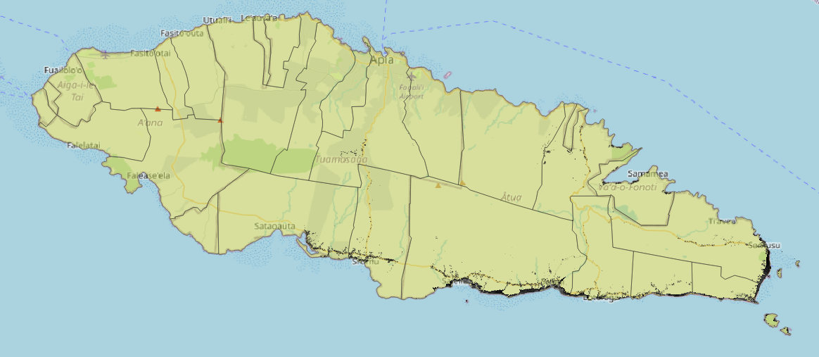
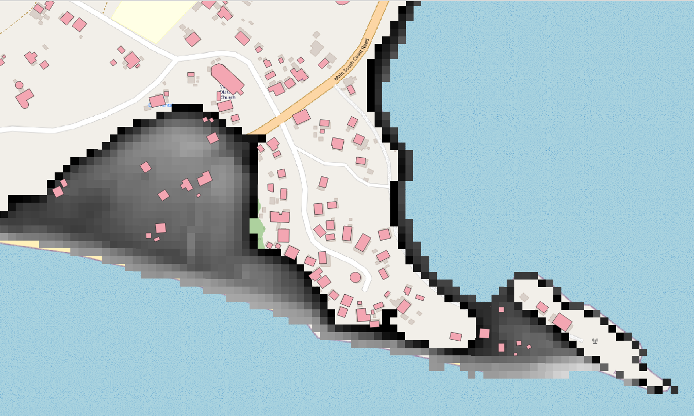
This is a screenshot of the geospatial data overlaid on an OpenStreetMap background. Looking at the data a little closer, without the area-layer, the building outlines and inundation hazard grid will look something like this:
RiskScape Projects
Within the unzipped directory, there is also a plain-text project.ini file.
This file is called the RiskScape project file, and it contains all the instructions that RiskScape needs to run your models.
Projects are a way to organize your RiskScape models, a bit like a work-space. You can use separate projects when you want to model different things.
We have already pre-populated this project file with example models. In later tutorials we will explain how to build your own models and project files from scratch.
RiskScape models
RiskScape models provide a flexible framework that let you customize aspects of the risk analysis workflow, such as using different input data, changing the analysis that is performed, or varying other assumptions that your model might make.
A high-level overview of the processing behind a simple RiskScape model looks like this:
The Python support in RiskScape lets you define exactly how the hazard will impact your element-at-risk, and what the resulting consequence will be. Later tutorials will explain more about how RiskScape’s geospatial matching works.
You can run a RiskScape model from the terminal using the riskscape model run command.
Running a model
Each RiskScape model has a unique name.
To start with, let’s look at a model called total-exposed.
To run this model, enter the following command into your terminal prompt.
riskscape model run total-exposed
The model should take a few seconds to run. RiskScape will display some progress statistics as it runs your model.
When RiskScape has finished it will display the output files produced, which contain the results of the model.
By default, RiskScape saves its results to an output/MODEL_NAME/TIMESTAMP/ sub-directory
within the current working directory, e.g. ./output/total-exposed/2022-08-16T15_07_20/event-impact.shp
Tip
If the RiskScape command produced an error, try checking that riskscape -V runs without
any errors, and that the current directory in your command prompt is in the unzipped getting-started
directory that contains the project.ini file.
This model produces two results files:
event-impact.shp: This shows the raw results from the model. The buildings from our input data are all still present, however, now each building also has ahazardvalue (the inundation depth, in metres) and aconsequencevalue (1or0, based on whether or not the building was exposed). Try opening this file in QGIS (or an equivalent application).summary.csv: This summarizes the effects of the tsunami, reporting the total number of buildings that were exposed. It also shows how many buildings were exposed to different tsunami inundation depths: 0-1m, 1-2m, and 3m+. Try opening the file in a spreadsheet application. You should see that 2059 out of 6260 buildings were exposed to the tsunami.
Tip
In QGIS, you can use rendering features,
such as graduated rendering
of the hazard attribute to better visualize the impact of the tsunami.
Note
If you are using ArcGIS, then you can also change the format of the model results.
E.g. riskscape model run total-exposed --format geopackage will produce a GeoPackage
results file instead of a shapefile. This .gpkg file should be more reliably
projected in ArcGIS.
Summarizing results by region
A useful way to view your model results is to aggregate them by a regional boundary of interest (in RiskScape we call this an area-layer). For example, you might be interested in how the impact from a hazard affects a specific district or particular towns.
We will look at how this tsunami hazard affects the different regions of south-eastern Upolu
by using a shapefile containing the Samoan electoral constituencies (Samoa_constituencies.shp).
Try running the exposed-by-region model using the following command.
riskscape model run exposed-by-region
This model produces an summary.csv results file in the output/exposed-by-region/TIMESTAMP/ sub-directory.
Try opening this file in a spreadsheet application.
This file contains the same basic results as the previous model, except that now the number of exposed buildings are
now broken by region, i.e. 749 in Falealili, 146 in Lotofaga, etc.
Note
Not every region in Samoa is included in these results because our building dataset only covers south-eastern Upolu.
Re-running models with different inputs
The customizable aspects of a RiskScape model are called the model’s parameters. Changing the model parameters lets you change the behaviour of the model on the fly.
For example, you may have several different hazard-layers that simulate different events, or represent the uncertainty associated with an event in different ways. RiskScape lets you run multiple different hazard-layers through the same model.
So far we have been using a GeoTIFF that models the tsunami inundation using a 50-metre grid resolution. However, we also have an alternative hazard-layer that models the tsunami using a 10-metre grid.
Let’s go back to our first total-exposed model, but try using the 10m grid hazard-layer in our model instead.
Copy and paste the following command exactly into your terminal:
riskscape model run total-exposed -p "input-hazards.layer=MaxEnv_All_Scenarios_10m.tif"
We will explain this command syntax more in later tutorials, but basically it changes the hazard-layer that the model uses.
Open the summary.csv file that was produced in a spreadsheet application.
You should see that the same total number of buildings were run through the model (6260), but now fewer buildings are reported as being exposed to the tsunami compared with the previous 50m grid (1568 vs 2059).
Note
These hazard-layers originally come from a research paper that reached this same finding. The paper concluded that the coarser 50m hazard grid tends to overestimate exposure.
Changing how results are reported
RiskScape models provide a flexible framework for analysing the impact of a hazard. By changing one parameter in the model, you can change how the results are reported. This can help you answer questions, such as:
What were the affected buildings used for (residential, industrial, commercial, etc)?
What types of building (timber, masonry, concrete, etc) were exposed?
If we exclude outbuildings, how many buildings were exposed?
How many residential buildings were exposed to 0.5m of inundation or greater?
The following RiskScape commands will alter the total-exposed model results to answer these questions.
Try copying and pasting each command one by one to re-run the model.
Open the resulting summary.csv file in a spreadsheet application and see what difference it has made to the results.
riskscape model run total-exposed -p "report-summary.group-by[0]=exposure.Use_Cat"

riskscape model run total-exposed -p "report-summary.group-by[0]=exposure.Cons_Frame"

riskscape model run total-exposed -p "report-summary.filter=exposure.Use_Cat != 'Outbuilding'"

riskscape model run total-exposed -p "report-summary.filter=hazard >= 0.5 and exposure.Use_Cat = 'Residential'"
Tip
The command syntax to change a model’s parameters can seem a bit fiddly initially. A simpler approach is to use the RiskScape wizard to build a new model with modified behaviour (later tutorials will explain how to do this). We have used the commands here to highlight that only one parameter in the model is changing.
Damage functions
So far we have simply been determining whether a building was exposed to the tsunami inundation or not. RiskScape lets you define your own Python function that will analyse the impact of the hazard. This means your RiskScape model can basically do whatever risk analysis you want it to.
We will now look at a model that uses the Samoa_Building_Fragility.py Python function to calculate
a damage state for each building.
The RiskScape function uses a log-normal Cumulative Distribution Function (CDF)
to determine the conditional probability (between 0 and 1.0) of a building being in a given damage state as a result of the tsunami inundation.
The following five different damage states are used, DS_1 through to DS_5:
Light: non-structural damage
Minor: significant non-structural and minor structural damage
Moderate: significant structural and non-structural damage
Severe: irreparable structural damage requiring demolition
Collapse: complete structural collapse
The building’s fragility (i.e. the shape of the log-normal CDF curve) will be different depending on the building’s construction material. For more background on how the fragility curve was determined, refer to the research paper Evaluating building exposure and economic loss changes after the 2009 South Pacific Tsunami.
The building-damage model then assigns an overall damage state to each building,
based on the calculated probabilities, using a weighted random choice.
To run this model, enter the following command into your terminal:
riskscape model run building-damage
This model produces two results files:
summary.csv: This shows the total number of buildings in each damage state, broken down by region.event-impact.shp: This contains each individual building, along with all its calculated damage state probabilities.
Tip
RiskScape lets you save the results in a variety of different formats. The default here has been shapefile, but you can also save geospatial results in GeoJSON, KML, GeoPackage, or PostGIS.
Summary
These examples show you some fairly simple uses of RiskScape in hazard modelling. You can also use RiskScape to build more complex models, such as:
Loss modelling. Instead of producing a damage state for each building, you could produce a loss value. This would let you calculate a total loss from an event.
Multi-hazard analysis. For example, you could assess the impact of earthquake shaking damage and tsunami inundation.
Geospatial processing. Instead of building data, you might have a roading dataset. You may want to buffer (enlarge) the width of the line-strings, or cut them into smaller 10m segments.
Probabilistic modelling. You may have hazard data that simulates hazard events across hundreds or thousands of years. RiskScape can use this data to calculate an Annual Average Loss, and other risk metrics.
If you want to learn more about the underlying concepts involved with building and running RiskScape models, you could now try the How RiskScape models work tutorial.